library(tidyverse)
library(sf)
library(units)
library(rnaturalearth)
library(knitr)
library(USAboundaries)
library(ggrepel)
library(gghighlight)

# Question 1
# 1.1 - Define a Projection
eqdc = '+proj=eqdc +lat_0=40 +lon_0=-96 +lat_1=20 +lat_2=60 +x_0=0 +y_0=0 +datum=NAD83 +units=m +no_defs'
region = data.frame(region = state.region, state_name = state.name)

# 1.2 - Get USA state boundaries
USConus = USAboundaries::us_states() %>%
  filter(!name %in% c("Puerto Rico", "Alaska", "Hawaii"))

#1.3 - Get country boundaries for Mexico, the United States of America, and Canada
Boundaries = rnaturalearthdata::countries110 %>%
  st_as_sf() %>%
  filter(name %in% c("Mexico", "United States of America", "Canada"))

# 1.4 - Get city locations from the CSV file
UScities = readr::read_csv("data/uscities.csv") %>%
  filter(!state_name %in% c("Puerto Rico", "Alaska", "Hawaii")) %>%
  st_as_sf(coords = c("lng", "lat"), crs = 4326) %>%
  st_filter(USConus, .predicate = st_intersects)

USConus = st_transform(USConus, eqdc)
Boundaries = st_transform(Boundaries, eqdc)
UScities = st_transform(UScities, eqdc)
# Question2
# 2.1 - Distance to USA Border (coastline or national) (km)
Border = st_union(USConus) %>%
  st_cast("MULTILINESTRING")

DistoB = UScities %>%
  mutate(dist_to_border = st_distance(UScities, Border),
         dist_to_border = units::set_units(dist_to_border, "km"),
         dist_to_border = units::drop_units(dist_to_border))

FurthesttoB = DistoB %>%
  slice_max(dist_to_border, n = 5) %>%
  select(city, state_name, dist_to_border) %>%
  st_drop_geometry()

knitr::kable(FurthesttoB,
             caption = "Furtherest Cities to Border",
             col.names = c("City Name", "State", "Distance(km)"))
Furtherest Cities to Border
| Dresden |
Kansas |
1012.317 |
| Herndon |
Kansas |
1007.750 |
| Hill City |
Kansas |
1005.147 |
| Atwood |
Kansas |
1004.734 |
| Jennings |
Kansas |
1003.646 |
# 2.2 - Distance to States (km)
Border2 = st_combine(USConus) %>%
  st_cast("MULTILINESTRING")

DistoB2 = UScities %>%
  mutate(dist_to_state = st_distance(UScities, Border2),
         dist_to_state = units::set_units(dist_to_state, "km"),
         dist_to_state = units::drop_units(dist_to_state))

FurthesttoS = DistoB2 %>%
  slice_max(dist_to_state, n = 5) %>%
  select(city, state_name, dist_to_state) %>%
  st_drop_geometry()

knitr::kable(FurthesttoS,
             caption = "Furtherest Cities to the States",
             col.names = c("City Name", "State", "Distance(km)"))
Furtherest Cities to the States
| Lampasas |
Texas |
308.9216 |
| Bertram |
Texas |
302.8190 |
| Kempner |
Texas |
302.5912 |
| Harker Heights |
Texas |
298.8125 |
| Florence |
Texas |
298.6804 |
# 2.3 - Distance to Mexico (km)
BorderMexico = Boundaries %>%
  filter(name %in% c("Mexico")) %>%
  st_cast("MULTILINESTRING")

DistoBMexico = UScities %>%
  mutate(dist_to_mexico = st_distance(UScities, BorderMexico),
         dist_to_mexico = units::set_units(dist_to_mexico, "km"),
         dist_to_mexico = units::drop_units(dist_to_mexico))

FurthesttoM = DistoBMexico %>%
  slice_max(dist_to_mexico, n = 5) %>%
  select(city, state_name, dist_to_mexico) %>%
  st_drop_geometry()


knitr::kable(FurthesttoM,
             caption = "Furtherest Cities to Mexico",
             col.names = c("City Name", "State", "Distance(km)"))
Furtherest Cities to Mexico
| Caribou |
Maine |
3250.334 |
| Presque Isle |
Maine |
3234.570 |
| Calais |
Maine |
3134.348 |
| Eastport |
Maine |
3125.624 |
| Old Town |
Maine |
3048.366 |
# 2.4 - Distance to Canada (km)
BorderCanada = Boundaries %>%
  filter(name %in% c("Canada")) %>%
  st_cast("MULTILINESTRING")

DistoBCanada = UScities %>%
  mutate(dist_to_canada = st_distance(UScities, BorderCanada),
         dist_to_canada = units::set_units(dist_to_canada, "km"),
         dist_to_canada = units::drop_units(dist_to_canada))

FurthesttoC = DistoBCanada %>%
  slice_max(dist_to_canada, n = 5) %>%
  select(city, state_name, dist_to_canada) %>%
  st_drop_geometry()

knitr::kable(FurthesttoC,
             caption = "Furtherest Cities to Canada",
             col.names = c("City Name", "State", "Distance(km)"))
Furtherest Cities to Canada
| Guadalupe Guerra |
Texas |
2206.455 |
| Sandoval |
Texas |
2205.641 |
| Fronton |
Texas |
2204.784 |
| Fronton Ranchettes |
Texas |
2202.118 |
| Evergreen |
Texas |
2202.020 |
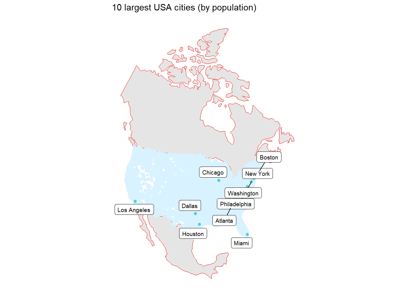
# Question3
# 3.1 - Data
LargeUScities = UScities %>%
  slice_max(population, n = 10)

ggplot()+
  geom_sf(data = Boundaries, aes(), col = "#f30100", size = 0.3) +
  geom_sf(data = DistoB2, col = "#d9f2ff", lty = 2) +
  geom_sf(data = LargeUScities, col = "#50d0d0", size = 1.5) +
  ggthemes::theme_map() +
  labs(title = "10 largest USA cities (by population)",
       x = "Longitude",
       y = "Latitude") +
  ggrepel::geom_label_repel(
    data = LargeUScities,
    aes(label = city, geometry = geometry),
    stat = "sf_coordinates",
    size = 2.5)
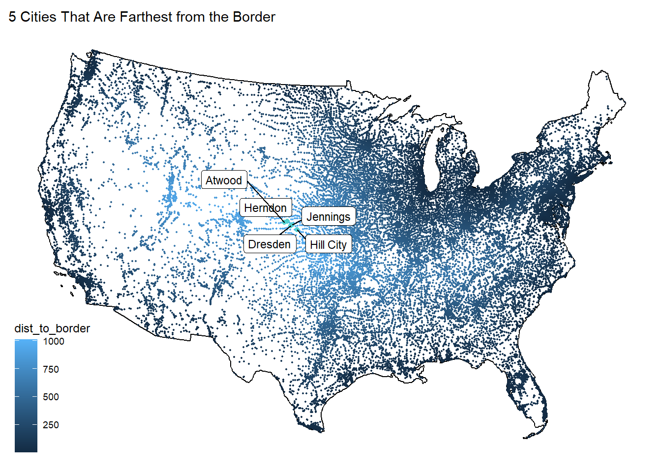
# 3.2 - City Distance from the Border
FurthesttoB3 = DistoB %>%
  slice_max(dist_to_border, n = 5) %>%
  select(city, state_name, dist_to_border)

ggplot() +
  geom_sf(data = Border, aes()) +
  geom_sf(data = DistoB, aes(col = dist_to_border), size = 0.3) +
  geom_sf(data = FurthesttoB3, col = "#50d0d0") +
  ggthemes::theme_map() +
  labs(title = "5 Cities That Are Farthest from the Border",
       x = "Longitude",
       y = "Latitude") +
  ggrepel::geom_label_repel(
    data = FurthesttoB3,
    aes(label = city, geometry = geometry),
    stat = "sf_coordinates",
    size = 3)
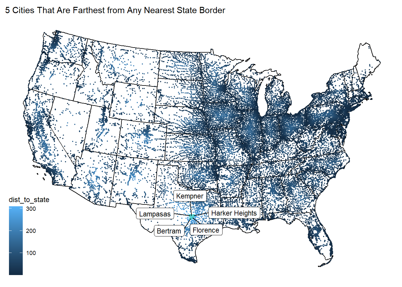
# 3.3 - City Distance from Nearest State
FurthesttoS3 = DistoB2 %>%
  slice_max(dist_to_state, n = 5) %>%
  select(city, state_name, dist_to_state)

ggplot() +
  geom_sf(data = Border2, aes()) +
  geom_sf(data = DistoB2, aes(col = dist_to_state), size = 0.3) +
  geom_sf(data = FurthesttoS3, col = "#50d0d0") +
  ggthemes::theme_map() +
  labs(title = "5 Cities That Are Farthest from Any Nearest State Border",
        x = "Longitude",
        y = "Latitude") +
  ggrepel::geom_label_repel(
    data = FurthesttoS3,
    aes(label = city, geometry = geometry),
    stat = "sf_coordinates",
    size = 3)
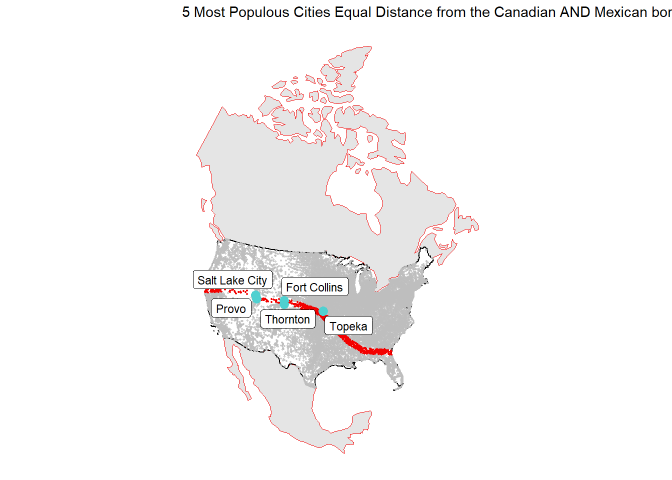
# 3.4 - Equidistant boundary from Mexico and Canada
Equidis = UScities %>%
  mutate(MCdis = abs(DistoBMexico$dist_to_mexico - DistoBCanada$dist_to_canada)) %>%
  select(MCdis, city, state_name, population)

LargeCities = Equidis %>%
  filter(MCdis <= 100)  %>%
  slice_max(population, n = 5)

ggplot() +
  geom_sf(data = Boundaries, aes(), col = "#f30100", size = 0.3) +
  geom_sf(data = Border) +
  geom_sf(data = Equidis, col = "#f30100", size = 0.3) +
  geom_sf(data = LargeCities, col = "#50d0d0", size = 3) +
  gghighlight::gghighlight(MCdis <= 100) +
  ggthemes::theme_map() +
  labs(title = "5 Most Populous Cities Equal Distance from the Canadian AND Mexican border ± 100 km.",
       x = "Longitude",
       y = "Latitude") +
  ggrepel::geom_label_repel(
    data = LargeCities,
    aes(label = city, geometry = geometry),
    stat = "sf_coordinates",
    size = 3)
#Question 4
# 4.1 - Quantifing Border Zone (Matches ACLU)
Totalpop = DistoB %>%
    mutate(totalpop = sum(population)) %>%
    select(id, totalpop) %>%
    st_drop_geometry()

Dangerpop = DistoB %>%
    filter(dist_to_border <= 160) %>%
    mutate(dangerpop = sum(population)) %>%
    left_join(Totalpop, by = "id")

numbers = length(Dangerpop$city)

Zone = Dangerpop %>%
  mutate(number = numbers) %>%
  select(number, dangerpop, totalpop) %>%
  st_drop_geometry() %>%
  mutate(percent = dangerpop / totalpop) %>%
  select(number, dangerpop, percent) %>%
  head(1)

knitr::kable(Zone, caption = "Quantifing Border Zone",
       col.names = c("Cities Number", "Population", "Percentage of Total"))
Quantifing Border Zone
| 12255 |
259876456 |
0.6543463 |
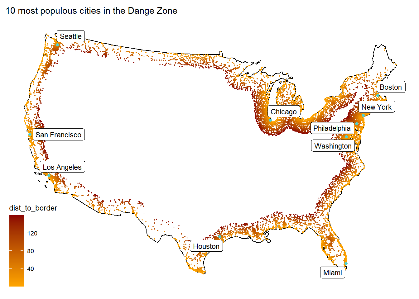
# 4.2 - Mapping Border Zone
ZoneCities = DistoB %>%
  filter(dist_to_border <= 160)

PopCities = ZoneCities %>%
  slice_max(population, n = 10)

ggplot() +
  geom_sf(data = ZoneCities, aes(col = dist_to_border), size = 0.3) +
  geom_sf(data = PopCities, col = "#50d0d0") +
  geom_sf(data = Border) +
  scale_color_gradient(low = "orange", high = "darkred") +
  gghighlight(dist_to_border <= 160) +
  ggthemes::theme_map() +
  labs(title = paste("10 most populous cities in the Dange Zone")) +
  ggrepel::geom_label_repel(
    data = PopCities,
    aes(label = city, geometry = geometry),
    stat = "sf_coordinates",
    size = 3)